SHAP Values Explained with Manchester City
SHAP Values Explained with Manchester City
SHAP values are based on Shapley values from game theory. These values help us fairly distribute payouts among players (or in our case, the importance of features in a model). In this context, we’re distributing “payouts” to the features that contribute to a machine learning model’s prediction.
- SHAP Values Explained with Manchester City
- The Football Analogy
- Marginal Contribution
- Drawbacks of Football Analogy
- Hard to Follow? Watch the Videos
- Kernel SHAP
 |
|---|
| *Guardiola giving bonuses but unsure how to rightfully distribute, you can see very accurate drawing of him :) * |
The Football Analogy
Let’s imagine Pep Guardiola, the coach of Manchester City, wants to distribute bonuses to four key players: Kevin De Bruyne, Raheem Sterling, Ilkay Gündoğan, and Riyad Mahrez. Pep wants to ensure the bonuses are distributed fairly based on each player’s contribution to the team’s success.
Pep and me know that without Kevin De Bruyne, the team wouldn’t have won the title. The challenge is to quantify how much each player contributed to the overall points the team earned.
And they want to give bonuses for all matches, UCL, FA CUP, League title, so don’t think if numbers doesn’t make sense.
 |
|---|
| Me advising Pep |
In order to make things easier, let’s assume 7 players are fixed at the beginning eleven, and they are having equal bonuses, so we don’t care about them. And we would like to only decide the bonuses of Raheem Sterling, Kevin De Bruyne, Sergio Aguare and Ilkay Gundogan, because they were the main driver of the championship title through the season.
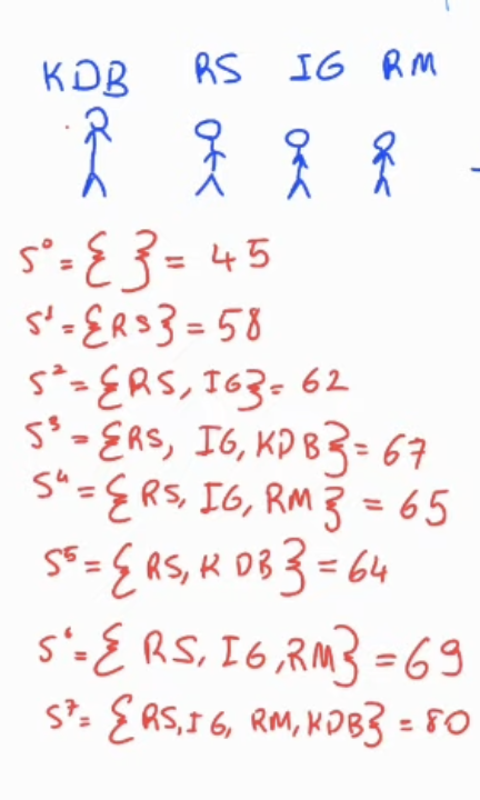
In order to quantify the effects of these players, I’m getting in front of my laptop to note all the points received with and without these players.
Matches played without these four players denoted as \(S^0= \left\{ \right\}\), matches played with only Raheem Sterling is denoted as \(S^0= \left\{ RS \right\}\). The points received on these matches are listed as below.
 |
|---|
| Points received with/out players |
Let’s calculate bonus of KDB, which is $\phi_{\text{KDB}}$.
SHAP values help us interpret the impact of each player (feature) on points received(individual predictions). By simulating the absence of a player (feature) (e.g., replacing it with its mean value), we can see how the model’s prediction changes.
We use the concept of marginal contributions. For each feature, we compare the model’s prediction with and without that feature across different subsets of features. The SHAP value for a feature is the weighted average of these marginal contributions.
\[ \phi_i = \sum_{S \subseteq N \setminus \{i\}} \frac{|S|!(|N|-|S|-1)!}{|N|!} \left[ v(S \cup \{i\}) - v(S) \right]\]Where:
-
\(\phi_i\) is the SHAP value for feature \(i\)
-
\(S\) is a subset of all features excluding \(i\)
-
\(N\) is the set of all features
-
\(v(S)\) is the model’s prediction for subset \(S\)
Marginal Contribution
What is the marginal contribution? Assume we have matches with Raheem Sterling and Ilkay Gundogan, and the points we receive on that matches:
\[ S=\left\{ RS,IG \right\}=62\]And, there are matches Raheem Sterling, Ilkay Gundogan and Kevin de Bruyne played together.
\[ S=\left\{ RS,IG,KDB \right\}=67\]So the marginal effect of adding KDB to the starting eleven for the specific RS IG combination \( \left\{ RS,IG \right\}\cup \left\{ KDB\right\}\) should be $67-62=5$, and this stands for the rightest side of the equation \( \left[ v(S \cup \{i\}) - v(S) \right]\).
What about the left side of the equation? What does that mean? \(\sum_{S \subseteq N \setminus \{i\}} \frac{|S|!(|N|-|S|-1)!}{|N|!}\)
- When calculating the SHAP value for a feature i to different subsets of features affects the model’s prediction.
- The factorial terms ensure that each subset’s contribution is weighted appropriately based on its size and the number of features not in the subset.
So it gives the proportion of all possible orderings of the features in which a particular subset S is considered.
And then you sum for all features. For the specific combination - \( \left\{ RS,IG \right\}\cup \left\{ KDB\right\}\) - we have
\[\frac{2!(4-2-1)!}{4!} = \frac{2}{24}\]Then, for the \( \left\{ RS,IG \right\}\cup \left\{ KDB\right\}\) we have
\[ \frac{2!(4-2-1)!}{4!} \left[ 67 - 62\right] = \frac{2}{24}*5 = \frac{10}{24}\]This is for specific combination, when we sum the all the contribution of KDB to first eleven, we will be able to calculate the bonus (shapley value) for $\phi_{\text{KDB}}$
Drawbacks of Football Analogy
When we choose football analogy with the them of Manchester City of 2021, it feels like every player positively contributed. This doesn’t necessarily true. Assume you do it for Brentford (average team on that season) and you may see some players negatively affected to the score.
Hard to Follow? Watch the Videos
I have three videos on explaining how SHAP works and how to calculate variables manually, what is the KernelSHAP and how to implement it on NumPy. Either you can watch videos, or skim through the post and then watch videos, it’s up to you. You’ll also have Python notebook that you can implement KernelSHAP from scratch at the end.
Kernel SHAP
Assume you have a model trained on 10 features, how would you test your model with 9 features? It is designed to take 10 inputs, right?
There’s a trick for this, called KernelSHAP which I explained in the Youtube video below along with Jupyter notebook with Numpy, blog post may come later depending on the demand.
Math of KernelSHAP:
Implementation of KernelSHAP through NumPy, Paper Explained
Implementation of KernelSHAP through NumPy: Jupyter Notebook and Repo Link